Chapter 21 Violations of Assumptions

Both t-tests and ANOVA make assumptions about the variable of interest. Namely, both assume:

The variable of interest approximately normally distributed
The variance of the variable is approximately the same in the groups being compared

When our data violate the assumptions of standard statistical tests, we have several options:

Ignore violations of the assumptions, especially with large sample sizes and modest violations
Transform the data (e.g., log transformation)
Nonparametric methods
Permutation tests

Libraries

library(tidyverse)
library(magrittr)
library(cowplot)
library(broom)

21.1 Graphical methods for detecting deviations from normality

As we have seen, histogram and density plot can highlight distributions that deviate from normality.

Look for: * distinctly non-symmetric spread – long tails, data up against a lower or upper limit * multiple modes * Varying bin widths (histograms) and the degree of smoothing (density plots) can both be useful.

Example data: Marine reserves

Example 13.1 in your text book describes a study aimed at understanding whether marine reserves are effective at preserving marine life. The data provided are “biomass ratios” between reserves and similar unprotected sites nearby. A ratio of one means the reserve and the nearby unprotected site had equal biomass; values greater than one indicate greater biomass in the rserve while values less than one indicate greater biomass in the unprotected site.

library(tidyverse)
library(magrittr)
library(cowplot)

marine.reserves <- read_csv("https://github.com/bio304-class/bio304-course-notes/raw/master/datasets/ABD-marine-reserves.csv")

ggplot(marine.reserves, aes(x = biomassRatio, y = ..density..)) +
  geom_histogram(bins=8, color='gray', alpha=0.5) + 
  stat_density(geom="line",
               adjust = 1.25,   # adjust is in multiples of smoothing bandwidth
               color = 'firebrick', size=1.5) +
  labs(x = "Biomass ratio", y = "Probability density")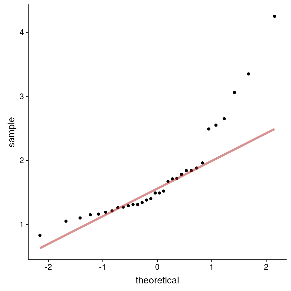

Both the histogram and the density plot suggest the biomass ratio distribution is strongly right skewed.

Normal probability plots

Normal probability plots are another visualization tools we saw previously for judging deviations from normality. If the observed data are approximately normally distributed, the scatter of points should fall roughly along a straight line with slope equal to the standard deviation of the data and intercept equal to the mean of the data.

ggplot(marine.reserves, aes(sample = biomassRatio)) + 
  geom_qq() + 
  geom_qq_line(color = 'firebrick', size = 1.5, alpha = 0.5)

21.2 Formal test of normality

There are number of formal tests of normality, with the “Shapiro-Wilk” test being among the most common. The Shapiro-Wilk test is essentially a formalization of the procedure we do by eye when judging a QQ-plot.

The null hypothesis for the Shapiro-Wilk test is that the data are drawn from a normal distribution. The test statistic for the Shapiro-Wilks tests is called \(W\), and it measures the ratio of sumed deviations from the mean for a theoretical normal relative to the observed data. Small values of W are evidence of departure from normality. As in all other cases we’ve examined, the observed \(W\) is compared to the expected sampling distribution of \(W\) under the null hypothesis to estimate a P-value. Small P-values reject the null hypothesis of normality.

shapiro.test(marine.reserves$biomassRatio)
#> 
#>  Shapiro-Wilk normality test
#> 
#> data:  marine.reserves$biomassRatio
#> W = 0.81751, p-value = 8.851e-05

21.3 When to ignore violations of assumptions

Estimation and testing of means tends to be robust to violation of assumptions of normality and homogeneity of variance. This robustness is a consequence of the Central Limit Theorem.

However, if “two groups are being compared and both differ from normality in different ways, then even subtle deviations from normality can cause errors in the analysis (even with fairly large sample sizes)” (W&S Ch 13).

21.4 Data transformations

A common approach to dealing with non-normal variables is to apply a mathematical function that transforms the data to more nearly normal distribution. Analyses and inferences are then done on the transformed data.

Log transformation: This widely-used transformation can only be applied to positive numbers, since log(x) is undefined when x is negative or zero. However, addition of a small positive constant can be used to ensure that all data are positive. For example, if a vector x includes negative numbers, then x + abs(min(x)) + 1 results in positive numbers that can be log transformed.

Arcsine square root transformation: \(p' = arcsin[\sqrt{p}]\) is often used when the data are proportions. If the original data are percentages, first divide by 100 to convert to proportions.

Square root transformation: \(Y' = \sqrt{Y + K}\), where \(K\) is a constant to ensure that no data points are negative. Results from the square root transformation are often very similar to log transformation.

Square transformation: \(Y' = Y^2\). This may be helpful when the data are skewed left. .

Antilog transformation: \(Y' = e^Y\) may be helpful if the square transformation does not resolve the problem. Only usable when all data points have the same sign. If all data points are less than zero, take the absolute value before applying the antilog transformation.

Reciprocal transformation: \(Y' = {\frac{1}{Y}}\) When data are right skewed, this transformation may be helpful. If all data points are less than zero, take the absolute value before applying the reciprocal transformation.

Example: log transformation to deal with skew

The biomass ratio variable in the marine reserves data is strongly right skewed. Let’s see how well a log transformation does in terms of normalizing this data:

ln.biomass.hist <- 
  ggplot(marine.reserves, aes(x = log(biomassRatio), y = ..density..)) + 
  geom_histogram(bins=8, color='gray', alpha=0.5) + 
  stat_density(geom="line",
               adjust = 1.25,   # adjust is in multiples of smoothing bandwidth
               color = 'firebrick', size=1.5) +
  labs(x = "ln[Biomass ratio]", y = "Probability density")

ln.biomass.qq <-
  ggplot(marine.reserves, aes(sample = log(biomassRatio))) + 
  geom_qq() + 
  geom_qq_line(color = 'firebrick', size = 1.5, alpha = 0.5) +
  labs(x = "ln[Biomass ratio]", y = "Theoretical quantiles")

plot_grid(ln.biomass.hist, ln.biomass.qq)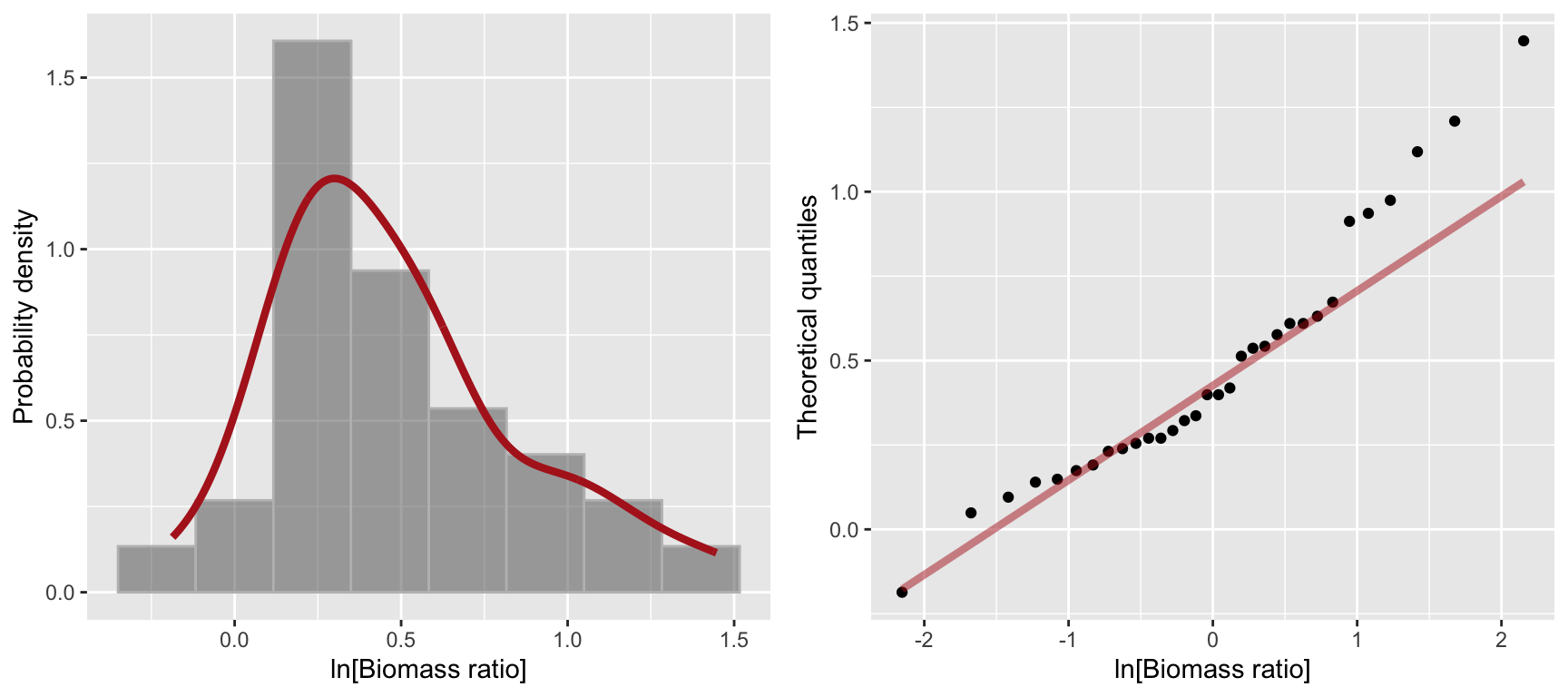

The log-transformed biomass ratio data is still a bit right skewed though not nearly as much as before. Applying the Shapiro-Wilk test to this transformed data, we fail to reject the null hypothesis of normality at \(\alpha = 0.05\).

shapiro.test(log(marine.reserves$biomassRatio))
#> 
#>  Shapiro-Wilk normality test
#> 
#> data:  log(marine.reserves$biomassRatio)
#> W = 0.93795, p-value = 0.06551

21.4.1 Confidence intervals and data transformations

Sometimes we need to transform our data before analysis, and then we want to know the confidence intervals on the original scale. In such cases, we back-transform the upper and lower CIs to the original scale of measurement.

Let’s calculate 95% CIs for the log-transformed biomass ratio data:

log.biomass.CI <- 
  marine.reserves %>%
  mutate(log.biomassRatio = log(biomassRatio)) %>%
  summarize(mean = mean(log.biomassRatio),
            sd = sd(log.biomassRatio),
            n = n(),
            SE = sd/sqrt(n),
            CI.low.log = mean - abs(qt(0.025, df = n-1)) * SE,
            CI.high.log = mean + abs(qt(0.025, df = n-1)) * SE) %>%
  select(CI.low.log, CI.high.log)

log.biomass.CI 
#> # A tibble: 1 x 2
#>   CI.low.log CI.high.log
#>        <dbl>       <dbl>
#> 1     0.3470      0.6112

This analysis finds the 95% CI around the mean of the log transformed data ranges is 0.347018, 0.6112365.

To understand the biological implications of this analysis, we back-transform the log data results to the original scale, computing the antilog by using function exp. After this, the back-transformed CI is now on the scale of \(e^{\log X} = X\).

Letting \(\mu'\) = mean(log.X), we have \(0.347 < \mu' < 0.611\) on the log scale.

On the original scale:

log.biomass.CI %>%
  # back-transform CI to original scale
  mutate(CI.low.original  = exp(CI.low.log),
         CI.high.original = exp(CI.high.log))
#> # A tibble: 1 x 4
#>   CI.low.log CI.high.log CI.low.original CI.high.original
#>        <dbl>       <dbl>           <dbl>            <dbl>
#> 1     0.3470      0.6112           1.415            1.843

Hence, 1.41 < geometric mean < 1.84.

The geometric mean equals \(\sqrt[n]{x_1 x_2 \cdots x_n}\), computed by multiplying all these n numbers together, then taking the \(n^{th}\) root.

Biologically, “this 95% confidence interval indicates that marine reserves have 1.41 to 1.84 times more biomass on average than the control sites do” (W&S 13.3)

21.5 Nonparametric tests

Non-parametric tests are ones that make no (or fewer) assumptions about the particular distributions from which the data of interest are drawn. Nonparametric tests are helpful for non-normal data distributions, especially with outliers. Typically, these tests use the ranks of the data points rather than the actual values of the data. Because they are not using all available data, nonparametric tests have lower statistical power than parametric tests. Nonparametric approaches still assume that the data are a random sample from the population.

We present here two common non-parametric alternatives to t-tests and ANOVA.

21.5.1 Mann-Whitney U-test: non-parametric alternative to t-test

When the normality assumption is not met, and none of the the standard mathematical transformations are suitable (or desirable), the Mann-Whitney U-test can be used in place of a two-sample \(t\)-test to compare the distribution of two groups. The Mann-Whitney U-test compares the data distribution of two groups, without requiring the normality assumptions of the two-sample t-test. The null hypothesis of this test is that the within-group data distributions are the same. Therefore, it is possible to reject the null hypothesis because the distributions differ, even if the means are the same. The Mann-Whitney U-test is sensitive to unequal variances or different patterns of skew. Therefore, this test should be used to compare distributions, not to compare means.

Confusingly, the Mann-Whitney U-test is also called the Mann–Whitney–Wilcoxon test. Do not confuse this with another test called the Wilcoxon signed-rank test.

Your textbook details the calculations involved, here we simply demonstrate the appropriate R function.

Example data: Sexual cannibalism in crickets

Example 13.5 in your textbook demonstrates the Mann-Whitney U-test with an application to a study of sexual cannabilism in sage crickets. During mating, male sage crickets offer their fleshy hind wings to females to eat. Johnson et al. (1999) studied whether female sage crickets are more likely to mate if they are hungry. They measured the time to mating (in hours) for female crickets that had be starved or fed. The null and alternative hypotheses for this comparison are:

\(H_0\): The distribution of time to mating is the same for starved and fed female crickets
\(H_A\): The distribution of time to mating differs between starved and fed female crickets

Here’s what the data look like:

crickets <- read_csv("https://github.com/bio304-class/bio304-course-notes/raw/master/datasets/ABD-cricket-cannibalism.csv")
#> Parsed with column specification:
#> cols(
#>   feedingStatus = col_character(),
#>   timeToMating = col_double()
#> )

ggplot(crickets, aes(x = timeToMating)) +
  geom_histogram(binwidth = 20, alpha = 0.75, fill = 'firebrick', color='black', center=10) +
  facet_wrap(~ feedingStatus, nrow=1)

As is apparent from the histograms, these data are decidedly non-normal. None of the standard mathematical transforms appear to work well in normalizing these data either.

To perform the Mann-Whitney U text, we use function wilcox.test (details here). This can take a data frame as input:

wilcox.test(timeToMating ~ feedingStatus, 
            alternative = "two.sided", paired = FALSE, data = crickets)
#> 
#>  Wilcoxon rank sum test
#> 
#> data:  timeToMating by feedingStatus
#> W = 88, p-value = 0.3607
#> alternative hypothesis: true location shift is not equal to 0

The test statistic \(W\) is the equivalent to the \(U\) test statistic of the Mann Whitney U-test. In this case, our observed value of \(U\) (\(W\)) is quite probable (\(p\) = 0.4) under the null hypothesis of no difference in the distributions between the two groups, therefore we fail to reject the null hypothesis.

21.5.2 Kruskal-Wallis test: non-parametric alternative to ANOVA

When there are more than two groups to compare, the non-parametric alternative to ANOVA is the Kruskal-Wallis Test. Like the Mann-Whitney U-test, the Kruskal-Wallis test is based on ranks rather than observed values. While the Kruskal-Wallis test does not assume the data are normally distributed, it still assumes the distributions of the variable of interest have similar shapes across the groups. The test statistic for the Kruskal-Wallis test is designated \(H\).

Example data: Daphnia resistance to cyanobacteria

This is from Assignment Problem 13.17 in Whitlock & Schluter.

Daphnia is a freshwater planktonic crustacean. Hairson et al. (1999) were interested in local adaptation of Daphnia populations in Lake Constance (bordering Germany, Austria, and Switzerland). Cyanobacteria, is a toxic food type that has increased in density in Lake Constance since the 1960s in response to increased nutrients. The investigators collected Daphnia eggs from sediments laid down during years of low, medium, and high cyanobacteria density and measured resistance to cyanobacteria in each group. Visual inspection of these data suggest they violate the normality assumptions of standard ANOVA.

daphnia <- read_csv("https://github.com/bio304-class/bio304-course-notes/raw/master/datasets/ABD-daphnia-resistance.csv")
#> Parsed with column specification:
#> cols(
#>   cyandensity = col_character(),
#>   resistance = col_double()
#> )

ggplot(daphnia, aes(x = resistance)) + 
  geom_histogram(bins=8, alpha = 0.75, fill = 'firebrick', color='black') + 
  facet_wrap(~ cyandensity)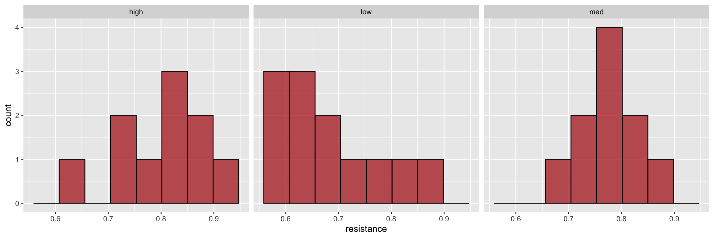

To carry out the Kruskal-Wallis test, and summarize the output in a data frame using broom::tidy we do:

kw.results <- kruskal.test(resistance ~ as.factor(cyandensity), daphnia)
tidy(kw.results)
#> # A tibble: 1 x 4
#>   statistic p.value parameter method                      
#>       <dbl>   <dbl>     <int> <chr>                       
#> 1     8.200 0.01658         2 Kruskal-Wallis rank sum test

Based on a the estimated P-value, we have evidence upon which to reject the null hypothesis of equal means at a Type I error rate of \(\alpha = 0.5\). However some caution is warranted as the shape of the distributions appear to be somewhat different among the groups.

Acknowledgements

Figures and examples from W&S Chap 13; lecture notes from T. Mitchell-Olds.