Chapter 17 Introduction to confidence intervals

Recall the concept of the sampling distribution of a statistic – this is simply the probability distribution of the statistic of interest you would observe if you took a large number of random samples of a given size from a population of interest and calculated that statistic for each of the samples.

You learned that the standard deviation of the sampling distribution of a statistic has a special name – the standard error of that statistic. The standard error of a statistic provides a way to quantify the uncertainty of a statistic across random samples. Here we show how to use information about the standard error of a statistic to calculate plausible ranges for a statistic of interest that take into account the uncertainty of our estimates. We call such plausible ranges Confidence Intervals.

17.1 Confidence Intervals

We know that given a random sample from a population of interest, the value of a statistic of interest is unlikely to be exactly equally to the true population value of that statistic. However, our simulations have taught us a number of things:

As sample size increases, the sample estimate of the given statistic is more likely to be close to the true value of that statistic
As sample size increases, the standard error of the statistic decreases

We will define an “X% percent confidence interval for a statistic of interest”, as an interval (upper and lower bound) that when calculated from a random sample, would include the true population value of the statistic of interest, X% of the time.

This quote from the NIST page on confidence intervals, which I’ve adapted to refer to any statistic, helps to make this concrete regarding confidence intervals:

As a technical note, a 95% confidence interval does not mean that there is a 95% probability that the interval contains the true [statistic]. The interval computed from a given sample either contains the true [statistic] or it does not. Instead, the level of confidence is associated with the method of calculating the interval … That is, for a 95% confidence interval, if many samples are collected and the confidence interval computed, in the long run about 95% of these intervals would contain the true [statistic].

The idea behind a 95% confidence interval is illustrated in the following figure:

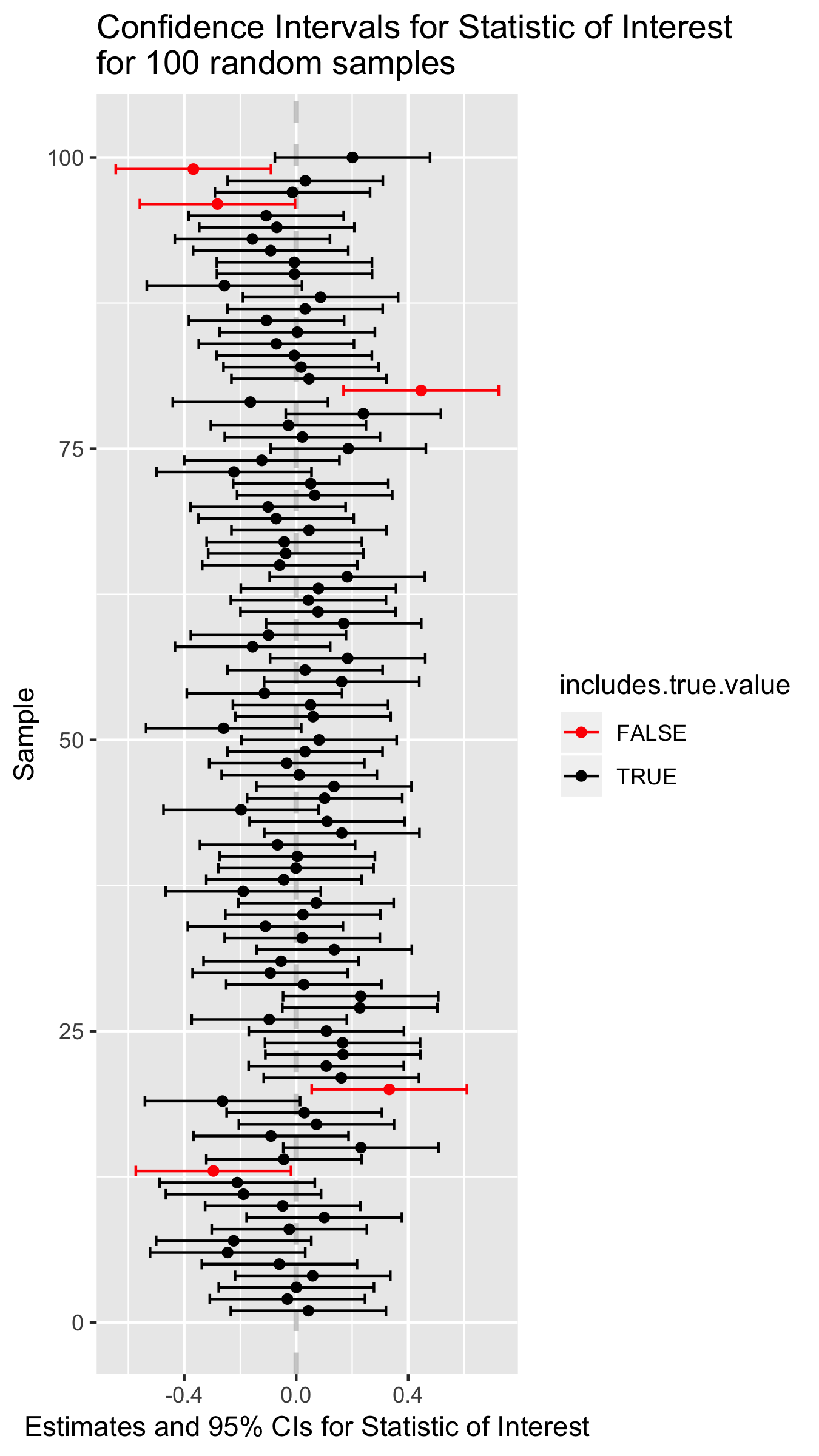
Figure 17.1: Point estimates and confidence intervals for a theoretical statistic of interest.

17.2 Generic formulation for confidence intervals

We define the \((100\times\beta)\)% confidence interval for the statistic \(\phi\) as the interval:

\[ CI_\beta = \phi_{n} \pm (z \times {SE}_{\phi,n}) \]

Where:

\(\phi_{n}\) is the statistic of interest in a random sample of size \(n\)
\({SE}_{\phi,n}\) is the standard error of the statistic \(\phi\) (via simulation or analytical solution)

And the value of \(z\) is chosen so that:

across many different random samples of size \(n\), the true value of the \(\phi\) in the population of interest would fall within the interval approximately \((100\times\beta)\)% of the time

So rather than estimating a single value of \(\phi\) from our data, we will use our observed data plus knowledge about the sampling distribution of \(\phi\) to estimate a range of plausible values for \(\phi\). The size of this interval will be chosen so that if we considered many possible random samples, the true population value of \(\phi\) would be bracketed by the interval in \((100\times\beta)\)% of the samples.

17.3 Example: Confidence intervals for the mean

To make the idea of a confidence interval more concrete, let’s consider confidence intervals for the mean of a normally distributed variable.

Recall that if a variable \(X\) is normally distributed in a population of interest, \(X \sim N(\mu, \sigma)\), then the sampling distribution of the mean of \(X\) is also normally distributed with mean \(\mu\), and standard error \({SE}_{\overline{X}} = \frac{\sigma}{\sqrt{n}}\):

\[ \overline{X} \sim N \left( \mu, \frac{\sigma}{\sqrt{n}}\ \right) \] In our simulation we will explore how varying the value of \(z\) changes the percentage of times that the confidence interval brackets the true population mean.

17.3.1 Simulation of means

In our simulation we’re going to generate a large number of samples, and for each sample we will calculate the sample estimate of the mean, and then quantify how much each sample mean differs from the true mean in terms of units of the population standard error of the mean. We’ll then use this information to calibrate the wide of our confidence intervals.

For the sake of simplicity we’ll simulate sampling from the “Standard Normal Distribution” – a normal distribution with mean \(\mu=0\), and standard deviation \(\sigma=1\).

First we load our standard libraries:

library(tidyverse)
library(magrittr)

Then we write our basic framework for our simulations:

rnorm.stats <- function(n, mu, sigma) {
  s <- rnorm(n, mu, sigma)
  df <- data_frame(sample.size = n,
                   sample.mean = mean(s),
                   sample.sd = sd(s),
                   pop.SE = sigma/sqrt(n))
}

And then use this to simulate samples of size 25.

set.seed(20180328) # initialize RNG seed

true.mean <- 0
true.sd <- 11
n <- 25

samples.25 <- 
  rerun(10000, rnorm.stats(n, true.mean, true.sd)) %>%
  bind_rows()

17.3.2 Distance between sample means and true means

We append a new column to our samples.25 data frame, which is the result of calculating the distance of each sample mean from the true mean, expressed in terms of units of the population standard error of the mean:

samples.25 <-
  samples.25 %>%
  mutate(z.pop = (sample.mean - true.mean)/pop.SE)

Since the sampling distribution of the mean of a normally distributed variable (\(N(\mu,\sigma)\)) is itself normally distributed (\(N(\mu, SE_{\overline{X}})\)), then the distribution of \(z = \frac{\overline{X} - \mu}{SE}\) is \(N(0,1)\). This is illustrated in the figure below where we compare our simulated z-scores to the theoretical expectation:

SE <- 1
ggplot(samples.25) +
  geom_histogram(aes(x = z.pop, y=..density..), bins=50) + 
  stat_function(fun = function(x){dnorm(x, mean=0, sd=SE)}, color="red")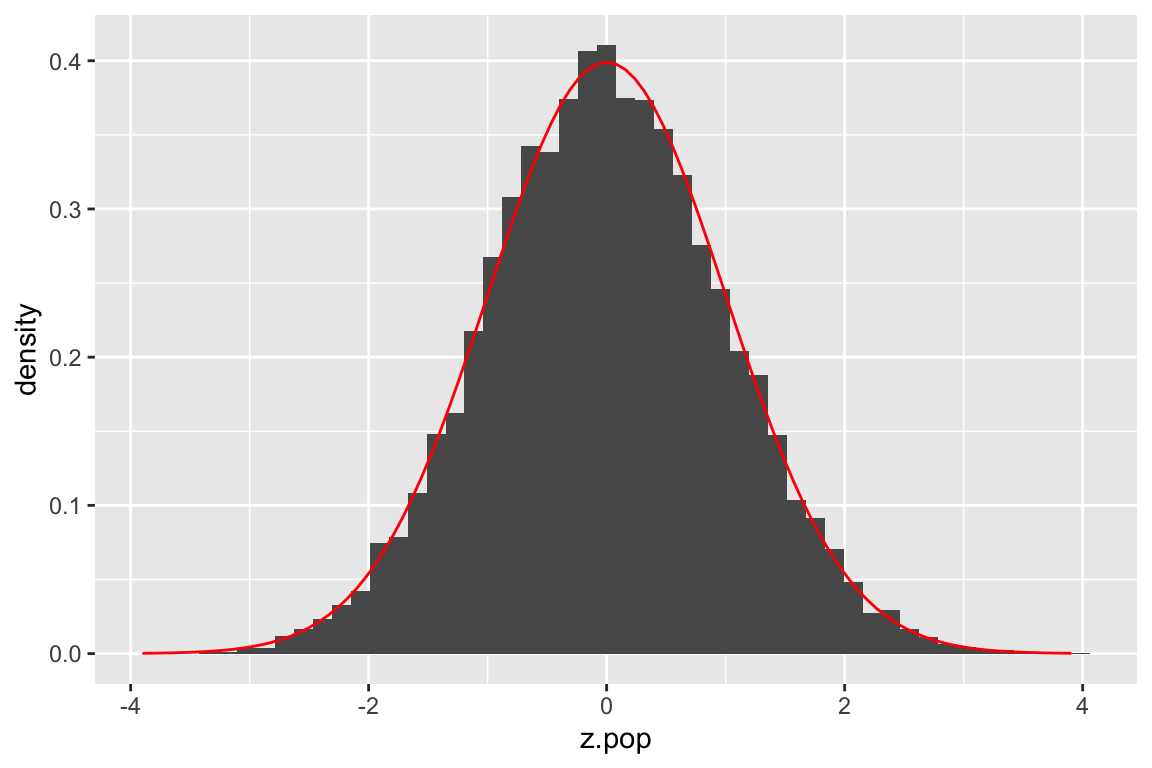

For a given value of \(z\) we can ask what fraction of our simulated means fall within \(\pm z\) standard errors of the true mean.

samples.25 %>%
  summarize(frac.win.1SE = sum(abs(z.pop) <= 1)/n(),
            frac.win.2SE = sum(abs(z.pop) <= 2)/n())
#> # A tibble: 1 x 2
#>   frac.win.1SE frac.win.2SE
#>          <dbl>        <dbl>
#> 1       0.6826       0.9549

We see that roughly 68% of our sample means are within 1 SE of the true mean; ~95% are within 2 SEs.

If we wanted to get exact multiples of the SE corresponding to different percentiles of the distribution of z-scores, based on the theoretical result (z scores ~ \(N(0,1)\)), we can use the qnorm() function:

frac.of.interest <- c(0.68, 0.90, 0.95, 0.99)

# we use 1 - frac to get left most critical value
# we divide by two here two account for area under left and right tails
left.critical.value <- qnorm((1 - frac.of.interest)/2, mean = 0, sd=1) 

data_frame(Percentile = frac.of.interest * 100,
           Critical.value = abs(left.critical.value))
#> # A tibble: 4 x 2
#>   Percentile Critical.value
#>        <dbl>          <dbl>
#> 1         68         0.9945
#> 2         90         1.645 
#> 3         95         1.960 
#> 4         99         2.576

17.3.3 Calculating a CI

If we knew the standard error of the mean for variable of interest, in order to a confidence interval we could simply look up the corresponding critical value for our percentile of interst in a table like the one above and calculate our CI as:

\[ \overline{X} \pm \text{critical value} \times SE_{\overline{X}} \]

For example, we see that the critical value for 95% CIs is ~1.96.

17.4 A problem arises!

If you’re a critical reader you should have noticed that calculating confidence intervals using the above formula presumes we know the standard error of the mean for the variable of interest. If we knew the standard deviation, \(\sigma\), of our variable, we could calculate this as \(SE_{\overline{x}} = \frac{\sigma}{\sqrt{n}}\) but in general we do not know \(\sigma\) either.

Instead we must estimate the standard error of the mean using our sample standard deviation:

\[ \widehat{SE}_{\overline{x}} = \frac{s_x}{\sqrt{n}} \]

This introduces another level of uncertainty and also a complication. The complication is due to the fact that for small samples, sample estimates of the standard deviation tend to be biased (smaller) relative to the true population standard deviation (see workbook Chapter 15).

In the assignment for this class session you will explore how we can deal with the fact of biased estimates of standard deviations for small samples, and how it effects our calculation of confidence intervals for the mean.