Chapter 14 Introduction to Sampling Distributions, Part I
14.2 In class experiments
14.2.1 Experiment 1
- Sample 10 grains of rice from the large population provided by the instructor
- Count the number of brown grains in your sample
- Enter your counts in this Google Sheets spreadsheet
- Once all the entire class has entered their data, download the spreadsheet as as CSV file, load it into R as a data frame (
rice) - Add a new column to the data frame that gives the proportion (relative frequency) of brown rice in each students sample
- Generate a frequency distribution plot for the proportion of brown rice
- Discuss as a class
Key points:
- We all did the same experiment
- We all sampled from the same population
- We all came up with slightly different estimates of the proportion of brown rice grains
- If we take all of our individual estimates and combine, we have a distribution of estimated proportions
14.2.2 Experiment 2
- Sample 30 grains of rice from the large population provided by the instructor
- Count the number of brown grains in your sample
- Add your new counts as additional rows to the Google Sheets spreadsheet
- Re-download and re-load the data, again estimating the proportion of brown rice for each student’s sample
- Generate a facetted plot giving the frequencing distribution for the proportion of brown rice in samples of size 10 and samples of size 30.
- Discuss as a class
Key points: - With larger sample sizes our estimates still very - But the spread of our estimates has decreased
14.3 Simulating sampling in R
Before we can simulate a sampling experiment in a computer we have to make some assumptions about the probability distribution of the variables we’re simulating.
To illustrate this let’s make explicit what’s going on in our rice grain experiment:
- We have a large population of rice grains
- A fraction, \(p\), of grains in that population are brown
- We draw \(n\) grains of rice from the population; all of the draws are independent
- We count the number of brown rice grains, recording the value as \(k\)
14.3.1 Binomial distribution
Under this scenario, what is the probability the we drew \(k\) brown grains from a sample of size \(n\), if the true proportion of brown grains is \(p\)?
It turns out we can solve this problem for a the following formula:
\[ P(k; n, p) = {n \choose k} p^k (1-p)^{n-k} \]
Where:
- \({n \choose k}\) is called the “binomial coefficient” and it gives the different combinations that would result in \(k\) successes (brown grains) in \(n\) draws. For example, in our rice experiment one combination for \(k=2\) would be: (brown, brown, white, white…); a second combination could be (brown, white, brown, white, white, …)
- \(p^k(1-p)^{n-k}\) is the probability of \(k\) successes (brown grains) and \((n-k)\) failures (white grains) for each of the combinations
The above formula is the “Probability Mass Function” (pmf) for the Binomial Distribution – it gives the probability of a particular outcome. The complete binomial distribution for \(n\) trials given a probability of success \(p\) is written as \(B(n,p)\) and is calculated by evaluating the probability mass function for all values of \(k\) from \(0,\ldots,n\).
14.3.1.1 Binomial distribution in R
R has a built-in function, dbinom() that calculates the probabability mass function of the binomial distribution at given values of \(k\). Tkae a moment to read the help on the dbinom() function in R.
To calculate the Binomial pmf for \(k=5, n = 10, p = 0.3\) we call dbinom() as so:
This tells us that if the true proportion of brown rice in the population is 0.3, about 10% of samples of size 10 will have 5 brown grains in them.
The dbinom() function can also take a vector of values of \(k\) as it’s first argument. Here we evaluate all values of \(k\) between 0 and 10, for the same scenario (\(n=10\) draws; probability of success \(p = 0.3\)), storing the results in a data frame.
k <- 0:10
binomial.ex1 <- data_frame(k = k,
                           probability = dbinom(k, 10, 0.3))
binomial.ex1
#> # A tibble: 11 × 2
#>        k probability
#>    <int>       <dbl>
#>  1     0 0.02825
#>  2     1 0.1211
#>  3     2 0.2335
#>  4     3 0.2668
#>  5     4 0.2001
#>  6     5 0.1029
#>  7     6 0.03676
#>  8     7 0.009002
#>  9     8 0.001447
#> 10     9 0.0001378
#> 11    10 0.000005905
And now plotting the distribution, using geom_col() which is like geom_bar() but that derives the height of the bars to plot directly from thes specified y aesthetic.
binomial.ex1 %>%
  ggplot(aes(x = k, y = probability)) +
  geom_col(width=0.25) +
  scale_x_continuous(breaks=1:10)
14.3.2 Sampling from the binomial distribution in R
To simulate sampling from the binomial distribution in R we can use the rbinom() function.
The arguments to rbinom() the number of samples, the number of draws in each sample, and the probability of success. For example, to simulate the single sample of size 10 that you generated at the beginning of class (making an assumption about the actual probability in the population) you would call rbinom() like so:
The value returned by rbinom() is the number of successes.
You can also specify more than one sample to be generated. For example, there are roughly 20 students in today’s class session. To simulate all of our 20 samples we can call rbinom() as so:
# 20 samples of size 10, where P(success) = 0.3
rbinom(20, 10, 0.3)
#>  [1] 1 3 3 2 5 6 2 1 3 2 3 3 3 3 5 3 6 2 5 2
Let’s repeat that, but for several thousand samples of size 10, and then plot the results in terms of the proportion of successes:
nsamples = 5000
ssize = 10
p = 0.3

df10 <- data_frame(ssize = rep(ssize, nsamples),
                   k = rbinom(nsamples, ssize, p),
                   estimated.p = k/ssize)

df10 %>%
  ggplot(aes(x = estimated.p)) +
  geom_histogram(bins=10)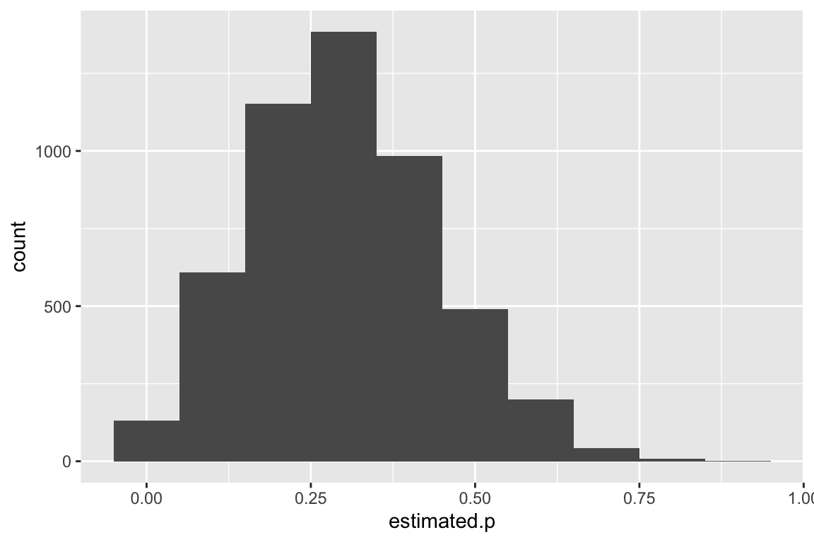
Here we’re plotting a distribution of the estimates of the proportion of successes (e.g. relative frequency of brown rice grains) in many samples of size 10.
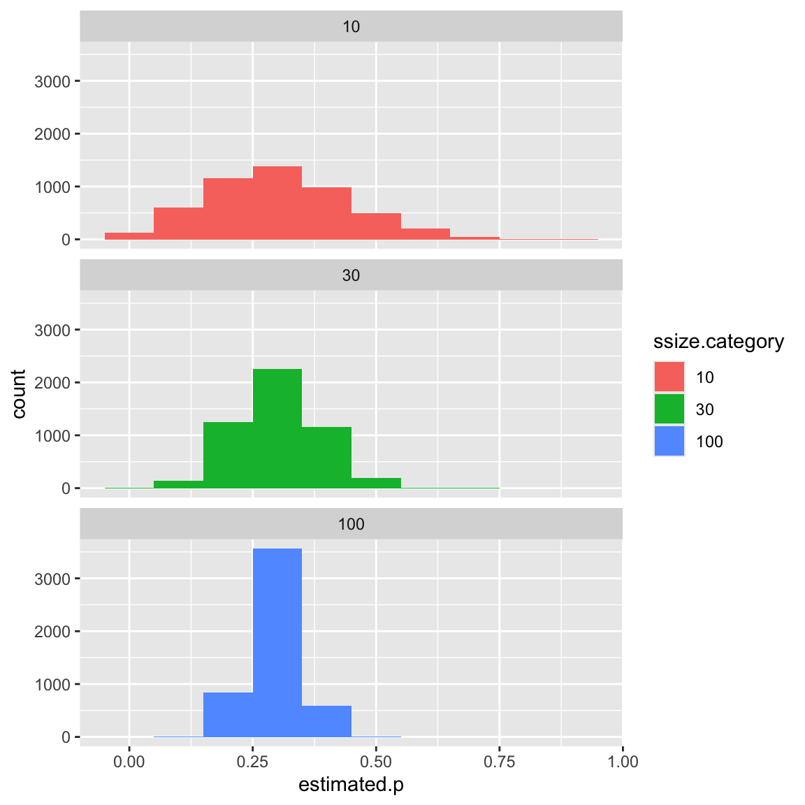
14.4 Distribution of estimates of the proportion
Repeat the simulation,but for samples of size 30:
nsamples = 5000
ssize = 30
p = 0.3

df30 <- data_frame(ssize = rep(ssize, nsamples),
                   k = rbinom(nsamples, ssize, p),
                   estimated.p = k/ssize)
Repeat the simulation, but for samples of size 100:
nsamples = 5000
ssize = 100
p = 0.3

df100 <- data_frame(ssize = rep(ssize, nsamples),
                   k = rbinom(nsamples, ssize, p),
                   estimated.p = k/ssize)
Combine the three data frames:
Plot distributions of estimates of \(p\) for different sample sizes:
df.combined %>%
  mutate(ssize.category = as.factor(ssize)) %>%
  ggplot(aes(x = estimated.p, fill = ssize.category)) +
  geom_histogram(bins=10) +
  facet_wrap(~ssize.category, ncol=1)