Chapter 19 Comparing sample means
19.1 Hypothesis test for the mean using the t-distribution
We consider three different situations for hypothesis tests regarding means.
19.2 One sample t-test
A one sample t-test is appropriate when you want to compare an observed sample mean to some a priori hypothesis about what the mean should be.
- \(H_0\): The mean of variable \(X\) equals \(\mu_0\) (some a priori value for the mean)
- \(H_A\): The mean of variable \(X\) does not equal \(\mu_0\)
19.2.1 One sample t-test, test statistic
To carry out a one sample t-test, first calculate the test statistic:
\[ t^{\star} = \frac{\overline{x} - \mu_0}{SE_{\overline{x}}} \]
where \(\overline{x}\) is the sample mean and \(SE_{\overline{x}}\) is the sample standard error of the mean (\(SE_{\overline{x}} = s_x/\sqrt{n}\)). In words, \(t^{\star}\) measures the difference between the observed mean, and the null hypothesis mean, in unit of standard error.
To calculate a P-value, we compare the test statistic to the t-distribution with the appropriate degrees of freedom to calculate the probability that you’d observe a mean value at least as extreme as \(\overline{x}\) if the null hypothesis was true. For a two-tailed test this is:
\[ P = P(t < -|t^\star|) + P(t > |t^\star|) \]
Since the t-distribution is symmetric, this simplifies to:
\[ P = 2 \times P(t > |t^\star|) \]
19.2.2 Assumptions of one sample t-tests
- Data are randomly sampled from the population
- The variable of interest is approximately normally distributed
19.2.3 Example: Gene expression in mice
You are an investigator studying the effects of various drugs on the expression of key genes that regulate apoptosis. The gene YFG1 is one such gene of interest. It has been previously established, using very sample sizes, that average expression level of the gene YFG1 in untreated (control) mice is 10 units.
You treat a sample of mice with Drug X, and measure the expression of the gene YFG1 following treatment. For a sample of five mice you observe the following expression values:
- YFG1 = {11.25, 10.5, 12, 11.75, 10}
You wish to determine whether the average expression of YFG1 in mice treated with the drug differs from control mice. The null and alternative hypotheses for this hypothesis test are:
- \(H_0\): the mean expression of YFG1 is 10
- \(H_A\): the mean expression of YFG1 does not equal 10
It’s relatively easy to calculate the various quantities of interest needed to carry out a one sided t-test:
library(tidyverse)

mu0 = 10  # mean under H0
mice.1sample <- data_frame(YFG1 = c(11.25, 10.5, 12, 11.75, 10))

YFG1.tstats <-
  mice.1sample %>%
  summarize(sample.mean = mean(YFG1),
            sample.sd = sd(YFG1),
            sample.se = sample.sd/sqrt(n()),
            df = n() - 1,
            mu0 = mu0,
            t.star = (sample.mean - mu0)/sample.se,
            P.value = 2 * pt(abs(t.star), df = df, lower.tail = FALSE))

YFG1.tstats
#> # A tibble: 1 × 7
#>   sample.mean sample.sd sample.se    df   mu0 t.star P.value
#>         <dbl>     <dbl>     <dbl> <dbl> <dbl>  <dbl>   <dbl>
#> 1        11.1    0.8404    0.3758     4    10  2.927 0.04295
Under the conventional \(\alpha = 0.05\), we reject the null hypothesis that the mean expression of YFG1 in mice treated with the drug is the same as the mean expression of YFG1 in control mice.
19.2.4 Confidence intervals for the mean
The hypothesis test using a one-side t-test we carried out above is approximately equivalent to asking if the null mean, \(\mu_0\), falls within the 95% confidence intervals estimated for the sample mean.
Recall that the \(100(1-\alpha)\)% confidence interval for the mean can be calculated as
\[ CI_\alpha = \overline{x} \pm (t_{\alpha/2,df} \times \widehat{SE}_{\overline{x}}) \]
Let’s modify the table of \(t\)-related stats we created in the previous code block to include the lower and upper limits of the 95% confidence interval for the mean:
YFG1.tstats <-
  YFG1.tstats %>%
  mutate(ci95.lower = sample.mean - abs(qt(0.025, df = df)) * sample.se,
         ci95.upper = sample.mean + abs(qt(0.025, df = df)) * sample.se)

YFG1.tstats
#> # A tibble: 1 × 9
#>   sample.mean sample.sd sample.se    df   mu0 t.star P.value ci95.lower
#>         <dbl>     <dbl>     <dbl> <dbl> <dbl>  <dbl>   <dbl>      <dbl>
#> 1        11.1    0.8404    0.3758     4    10  2.927 0.04295      10.06
#> # ℹ 1 more variable: ci95.upper <dbl>
If we wanted to crate a figure illustrating our 95% CI for the mean of YFG1 following drug treatment, relative to the mean under the null hypothesis we can use the geom_pointrange() function to draw the interval (for more info on geom_pointrange() and related functions see the ggplot2 documentation).
YFG1.tstats %>%
  ggplot() +
  geom_pointrange(aes(x = 1,
                      y = sample.mean,
                      ymin = ci95.lower, ymax = ci95.upper)) +
  scale_x_continuous(breaks=c(1), labels=c("Drug X")) +
  geom_hline(yintercept = mu0, color='red', linetype = 'dashed') +
  ylim(0,15) +
  labs(x = "", y = "Mean(YFG1)",
       title = "Sample mean and 95% CI for expression of YFG1 in treated mice",
       subtitle = "Red line indicates mean expression in control mice.") +
  theme_classic() +
  theme(plot.title = element_text(size = 12),
        plot.subtitle = element_text(size = 10))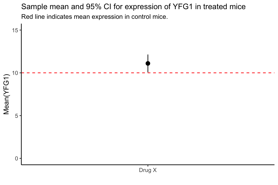
19.3 The t.test function in R
The built-in t.test() function will take care of the all the calcuations we did by hand above.
For a one sample t-test t.test we need to pass in the variable of interest, and the null hypothoses mean value, mu:
YFG1_t.test <- t.test(mice.1sample$YFG1, mu = 10)
YFG1_t.test
#>
#>  One Sample t-test
#>
#> data:  mice.1sample$YFG1
#> t = 2.9268, df = 4, p-value = 0.04295
#> alternative hypothesis: true mean is not equal to 10
#> 95 percent confidence interval:
#>  10.05652 12.14348
#> sample estimates:
#> mean of x
#>      11.1
The broom::tidye() function defined in the “broom” package is a convenient way to display the output of many model tests in R. Load the broom (install it first if need be) and use tidy() to represent the information returned by t.test() as a data frame:
19.4 Two sample t-test
We use a two sample t-test to analyze the difference between the means of the same variable measured in two different groups or treatments. It is assumed that the two groups are independent samples from two populations.
\(H_0\): The mean of variable \(X\) in group 1 is the same as the mean of \(X\) in group 2, i.e., \(\overline{x}_1 = \overline{x}_2\). This is equivalent to \(\overline{x}_1 - \overline{x}_2 = 0\).
\(H_A\): The mean of variable \(X\) in group 1 is not the same as the mean of \(X\) in group 2, i.e. \(\overline{x}_1 \neq \overline{x}_2\). This is equivalent to \(\overline{x}_1 - \overline{x}_2 \neq 0\).
19.4.1 Standard error for the difference in means
In a two-sample t-test, we have to account for the uncertainty associated with the means of both groups, which we express in terms of the standard error of the difference in the means between the groups:
\[ SE_{\overline{x}_1 - \overline{x}_2} = \sqrt{s^2_p\left(\frac{1}{n_1} + \frac{1}{n_2} \right)} \]
where
\[ s^2_p = \frac{df_1 s_1^2 + df_2 s_2^2}{df_1 + df_2} \]
\(s^2_p\) is called the “pooled sample variance” and is a weighted average of the sample variances, \(s_1^2\) and \(s_2^2\), of the two groups.
19.4.2 Two sample t-test, test statistic
Given the standard error for the difference in means between groups as defined above, we define our test statistic for a two sample t-test as:
\[ t^\star = \frac{(\overline{x}_1 - \overline{x}_2)}{SE_{\overline{x}_1 - \overline{x}_2}} \]
The degrees of freedom for this test statistic are:
\[ df = df_1 + df_2 = n_1 + n_2 - 2 \]
19.4.3 Assumptions of two sample t-test
- Data are randomly sampled from the population
- Paired differences are normally distributed
- Standard deviation is the same in both populations
19.4.4 Example: Comparing the effects of two drugs
You treat samples of mice with two drugs, X and Y. We want to know if the two drugs have the same average effect on expression of the gene YFG1. The measurements of YFG1 in samples treated with X and Y are as follows:
- X = {11.25, 10.5, 12, 11.75, 10}
- Y = {8.75, 10, 11, 9.75, 10.5}
For simplicity, we skip the “by-hand” calculations and simply use the built-in t.test function.
mice.2sample <- data_frame(YFG1_X = c(11.25, 10.5, 12, 11.75, 10),
                           YFG1_Y = c(8.75, 10, 11, 9.75, 10.5))

ttest.2sample <-
  t.test(mice.2sample$YFG1_X, mice.2sample$YFG1_Y)

ttest.2sample
#>
#>  Welch Two Sample t-test
#>
#> data:  mice.2sample$YFG1_X and mice.2sample$YFG1_Y
#> t = 2.0605, df = 7.9994, p-value = 0.07331
#> alternative hypothesis: true difference in means is not equal to 0
#> 95 percent confidence interval:
#>  -0.1310858  2.3310858
#> sample estimates:
#> mean of x mean of y
#>      11.1      10.0
This output provides information on:
- the data vectors used in this analysis
- t, df, and p-value
- the alternative hypothesis
- the 95% CI for the difference between the group means
- the group means
Using a type I error cutoff of \(\alpha = 0.05\), we fail to reject the null hypothesis that the mean expression of YFG1 is different in mice treated with Drug X versus those treated with Drug Y.
As we saw previously, broom::tidy() is a good way to turn the results of the t.test() function into a convenient table for further computation or plotting:
19.4.5 Specifying t.test() in terms of a formula
In the example above, our data frame included two columns for YFG1 expression values – YFG1_X and YFG1_Y – representing the expression measurements under the two drug treatments. This is not a very “tidy” way to organize our data, and is somewhat limiting when we want to create plots and do other analyses. Let’s use some of the tools we’ve seen earlier for tidying and restructuring data frames to unite these into a single column, and create a new column indicating treatment type:
mice.long <-
  mice.2sample %>%
  gather(expt, expression) %>%
  separate(expt, c("gene", "treatment"), sep="_")

head(mice.long)
#> # A tibble: 6 × 3
#>   gene  treatment expression
#>   <chr> <chr>          <dbl>
#> 1 YFG1  X              11.25
#> 2 YFG1  X              10.5
#> 3 YFG1  X              12
#> 4 YFG1  X              11.75
#> 5 YFG1  X              10
#> 6 YFG1  Y               8.75
Using this “long” data frame we can carry out the t.test as follows:
ttest.2sample <- t.test(expression ~ treatment, data = mice.long)
ttest.2sample
#>
#>  Welch Two Sample t-test
#>
#> data:  expression by treatment
#> t = 2.0605, df = 7.9994, p-value = 0.07331
#> alternative hypothesis: true difference in means between group X and group Y is not equal to 0
#> 95 percent confidence interval:
#>  -0.1310858  2.3310858
#> sample estimates:
#> mean in group X mean in group Y
#>            11.1            10.0
This long version of the data is also more easily used for calculating confidence intervals of the mean for each treatment, and for plotting as illustrated bloew
ci.by.treatment <-
  mice.long %>%
  group_by(treatment) %>%
  summarize(mean = mean(expression),
            se = sd(expression)/sqrt(n()),
            tcrit = abs(qt(0.025, df = n() - 1)),
            ci.low = mean - tcrit * se,
            ci.hi = mean + tcrit * se)

ci.by.treatment
#> # A tibble: 2 × 6
#>   treatment  mean     se tcrit ci.low ci.hi
#>   <chr>     <dbl>  <dbl> <dbl>  <dbl> <dbl>
#> 1 X          11.1 0.3758 2.776 10.06  12.14
#> 2 Y          10   0.3791 2.776  8.947 11.05
Here I combine the raw expression measurements and mean and confidence intervals into a single plot:
mice.long %>%
  ggplot(aes(x = treatment, y = expression, color=treatment)) +
  geom_point(alpha = 0.35, shape=17) +
  geom_pointrange(data = ci.by.treatment,
                  aes(x = treatment, y = mean,
                      ymin = ci.low, ymax= ci.hi)) +
  labs(x = "Drug Treatment", y = "Expression") +
  theme_classic() +
  theme(plot.caption = element_text(size=8))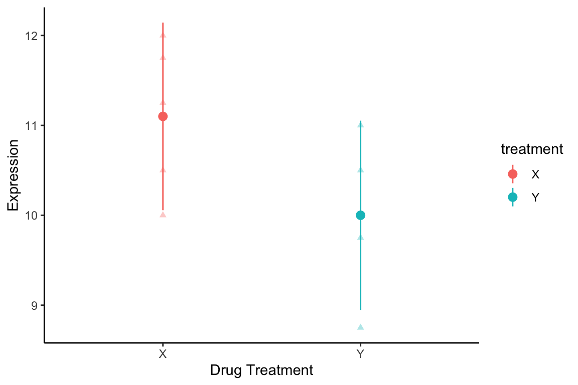
Figure 19.1: Expression of YFG1 for different drug treatments. Triangles are individual measurements. Circles and lines indicate group means and 95% CIs of means.
19.5 Paired t-test
In a paired t-test there are two groups/treatments, but the samples in the two groups are paired or matched. This typically arises in “before-after” studies where the same individual/object is measured at different time points, before and after application of a treatment. The repeated measurement of the same individual/object means that we can’t treat the two sets of observations as independent. Null and alternative hypotheses are thus typically framed in terms of a mean difference between time points/conditions
\(H_0\): The mean difference of variable \(X\) in the paired measurements is zero, i.e., \(\overline{D} = 0\) where \(D = X_\text{after} - X_\text{before}\)
\(H_A\): The mean difference of variable \(X\) in the paired measurements is not zero, i.e., \(\overline{D} \neq 0\)
19.5.1 Paired t-test, test statistic
- Let the variable of interest for individual \(i\) in the paired conditions be designated \(x_{i,\text{before}}\) and \(x_{i, \text{after}}\)
- Let \(D_i = x_{i, \text{after}} - x_{i, \text{before}}\) be the paired difference for individual \(i\)
- Let \(\overline{D}\) be the mean difference and \(s_D\) be the standard deviation of the differences
- The standard error of the mean difference is \(SE(\overline{D}) = \frac{s_D}{\sqrt{n}}\)
The test statistic is thus: \[ t^\star = \frac{\overline{D}}{SE(\overline{D})} \]
Under the null hypothesis, this statistic follows a t-distribution with \(n-1\) degrees of freedom.
19.5.2 Assumptions of paired t-test
- Data are randomly sampled from the population
- Paired differences are normally distributed
19.5.3 Paired t-test, example
You measure the expression of gene YFG1 in five mice. You then treat those five mice with drug Z and measure gene expression again.
- YFG1 expression before treatment = {12, 11.75, 11.25, 10.5, 10}
- YFG1 expression after treatment = {11, 10, 10.50, 8.75, 9.75}
mice.paired <- data_frame(YFG1.before = c(12, 11.75, 11.25, 10.5, 10),
                          YFG1.after = c(11, 10, 10.50, 8.75, 9.75))

t.test(mice.paired$YFG1.before, mice.paired$YFG1.after,
       paired = TRUE)
#>
#>  Paired t-test
#>
#> data:  mice.paired$YFG1.before and mice.paired$YFG1.after
#> t = 3.773, df = 4, p-value = 0.01955
#> alternative hypothesis: true mean difference is not equal to 0
#> 95 percent confidence interval:
#>  0.2905341 1.9094659
#> sample estimates:
#> mean difference
#>             1.1
Using a type I error cutoff of \(\alpha = 0.05\), we reject the null hypothesis of no difference in the average expression of YFG1 before and after treatment with Drug Z.
19.6 The fallacy of indirect comparison
WS 12.5 considers an example where baby photos were compared to photos of their mother, father, and several unrelated pictures. Volunteers were asked to identify the mother and father of each baby, and the accuracy of their choices was compared between mothers and fathers. In Fig. 12.5-1 (below), the horizontal line shows the null hypotheses expected for random guessing, while means and 95% CIs are shown for mothers and fathers. The success rate for picking fathers was significantly better than random expectation, while the CI for mothers overlapped the null expected value. Given these CIs, the authors of the study concluded that babies resemble their fathers more than their mothers.
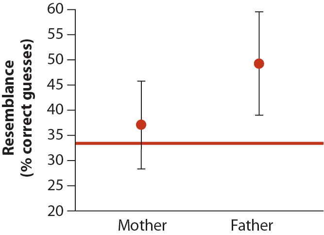
This is an example of the fallacy of indirect comparison: “Comparisons between two groups should always be made directly, not indirectly by comparing both to the same null hypothesis” WS 12.5.
19.6.1 Interpreting confidence intervals in light of two sample t-tests
Figure 12.6-1 from WS (below) considers the relationship between overlap of confidence intervals and significant difference between groups (\(H_0\): group means do not differ). Shown are group means and their 95% confidence intervals in three cases. (a) When 95% CIs do not overlap, then group means will be significantly different. (b) When the confidence interval of one group overlaps the mean value for the other group, then the groups are not significantly different. Finally, (c) when the confidence intervals overlap each other, but they do not overlap the mean of the other group, then the result of the hypothesis test is unclear.
In each case, figures with confidence intervals are helpful, but it is the P-value from our test of \(H_0\) that provides clear indication for our statistical conclusions.
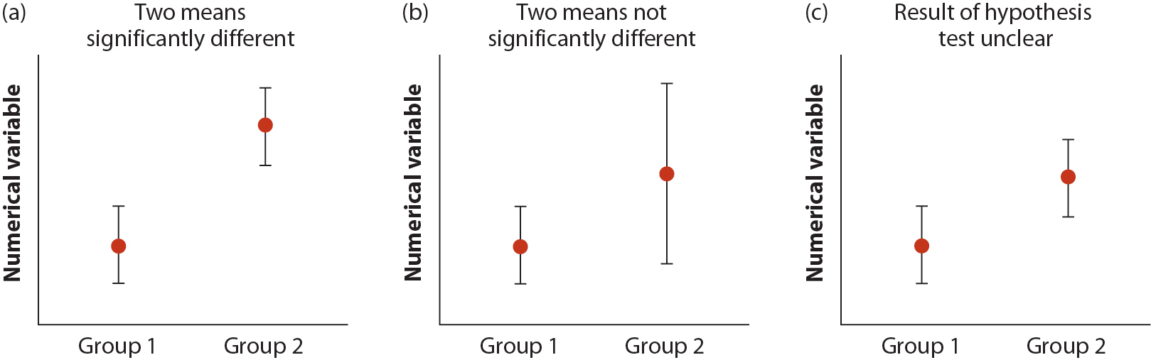
Figure 19.2: Figure from Whitlock and Schluter, Chapter 12.
19.7 Summary table for different t-tests
Here is a summary table giving the test statistic and degrees of freedom for each of the different types of t-tests described above. Notice that they all boil down to a difference of two means, expressed in units of standard error. The associated P-value associated with each test is thus a measure of how surprising that scaled difference in means is under the null model.
| test statistic | df | |
|---|---|---|
| one-sample | \(\frac{\overline{x}-\mu_0}{SE_{\overline{x}}}\) | \(n-1\) |
| two-sample | \(\frac{\overline{x}_1-\overline{x}_2}{SE_{(\overline{x}_1-\overline{x}_2})}\) | \(n_1 + n_2 - 2\) |
| paired | \(\frac{\overline{D}-0}{SE_{\overline{D}}}\) | \(n-1\) |