Chapter 13 Introduction to Probability
The exposition here largely follows that in Chapter 5 of Whitlock & Schluter.
13.1 Terms
Outcome – the result of a process or experiment
Random Trial – a process or experiment that has two or more possible outcomes whose occurence can not be predicted with certainty
Event – a subset of the possible outcomes of a random trial
13.1.1 Examples of random trials, outcomes, and events
13.1.1.1 Random trials
Classic examples of random trials
- flipping a coin
- rolling a die
- choosing a shuffled deck
- picking three balls, without replacement, from an urn filled with 3 white and 2 black balls
Biological examples of random trials
- Determining the sex of offspring in a genetic cross
- Weight loss/gain following treatment with a drug
- Count the plant species in one acre of forest
13.1.1.2 Outcomes
Classic examples:
- Coins: heads or tails
- Dice: The numbers \(1\) to \(n\), where \(n\) is the number of sides on the die that was thrown
- Cards: Any of the numbered or face cards and their suits
- Balls and urns: the number of black and white balls drawn
Biological examples:
- Sex of offspring: male and female
- Weight loss/gain: positive and negative real numbers in an interval
- Species: integers values \(\geq 0\)
13.1.1.3 Events
Classic examples:
- Coins: heads or tails (the events are the outcomes when the experiment is a single flip)
- Dice: rolled a specific number, rolled an event number, rolled a number greater than three, etc
- Cards: drew a face card, drew a heart, drew an ace of hearts, etc
- Balls and urns: all white balls, only one white ball, etc
Biological examples:
- Sex of offspring: male or female
- Weight loss/gain: lost weight, lost more than 5 lbs, gained between 10 and 20 lbs, etc
- Species: counted 10 species, counted more than 25 species, etc
13.2 Frequentist definition of probability
Probability of an event – the proportion of times the event would occur if we repeated a random trial an infinite (or very large) number of times under the same conditions.
To indicate the probability of an event \(A\), we write \(P(A)\)
The probability of all possible outcomes of a random trial must sum to one.
The complement of an event is all the possible outcomes of a random trial that are not the event. Let \(A^c\) indicate the complement of the event \(A\). Then \(P(A^c) = 1 - P(A)\)
13.2.1 Examples: Probability
13.2.1.1 Classic examples
In classic probabilistic examples, where we understand (approximately) the physical constraints and symmetries of a random trial, we can often assign theoretical probabilities:
Coins: With a fair coin, the probability of each face is 0.5
Dice: Given a fair 20-side die, the probability of rolling a 15 or better is 6/20 = 0.3
Cards: In randomly shuffled standard (French) 52-card deck, the probability of drawing a heart is 13/54 = 0.25; the probability of getting an ace is 4/52 = ~0.077; the probability of drawing the ace of hearts is 1/52 = ~0.0192 The probability of not drawing an ace is 1 - 1/52 = ~0.9808
Balls and urns: If you make three draws (without replacement) from an urn filled with three white and two black balls, the probability of drawing three white balls is 0.1. We’ll illustrate how to calculate this below.
13.2.1.2 Biological examples
For real-world examples, we can not usually invoke physical symmetries to assign theoretical probabilities a prioiri to an event (though sometimes we’ll use such symmetries when stating “null hypotheses”; more on this in a later lecture),
- Sex of offspring in humans: In human populations, the sex ratio at birth is not 1:1. The probability of a child being male is ~0.512, and the probability of having a female child is ~0.488. This surprising deviation from the 1:1 ratio is well documented. Additional factors contributes to further deviations in actual human populations. See for example Hesketh and Xing (2006), Abnormal sex ratios in human populations: causes and consequences. PNAS 103(36):13271-5.
13.3 Probability distribution
Probability distribution – A list, or equivalent representation, of the probabilities of all mutually exclusive outcomes of a random trial. Two events are mutually exclusive if than cannot both occur at the same time. The total probabilities in a probability distribution sums to 1.
For most cases of biological interest, probability distributions are unknowable and thus we use relative frequency distributions to estimate the underlying probability distributions of interest (relative frequencies are sometimes referred to as empirical probabilities).
Referring back to our earlier “frequentist definition”, another way of thinking about a probability distribution is as relative frequency distribution as the number of observations approaches the size (in some cases infinite) of the population under study (using the broad definition of “population” discussed several lectures ago)
13.3.1 Discrete probability distribution
Discrete probability distribution – the probability of each possible value of a discrete variable. Discrete probability distributions apply to categorical variables, ordinal variables, and discrete numerical variables. The total probabilities must sum to one.
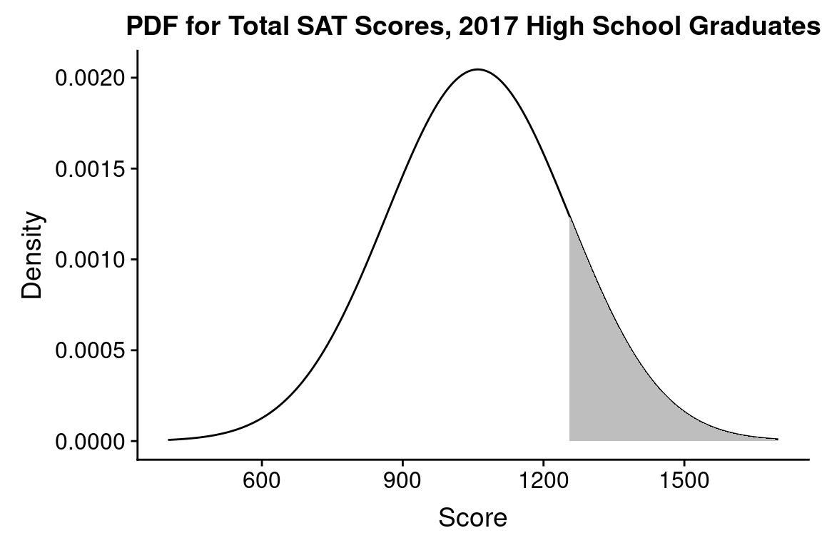
Figure 13.1: Discrete probability distributions. A) Probability distribution for a single roll of a fair 6-sided die; B) Probability distribution for the number of white balls observed in three draws, without replacement, from an urn filled with 3 white balls and 2 black balls.
13.3.2 Continuous probability distribution
Continuous probability distribution – for continuous numerical variables we do not assign probability to specific numerical values, but rather to numerical intervals. We represent a continuous probability distribution using a “Probability Density Function” (PDF). The integral of a PDF over an interval gives the probability that the variable represented by that PDF lies within the specified interval.
. The probability that a randomly chosen student got a score better than 1255 is represented by the shaded area; P(Score > 1255) = 0.1587.](bio304-book_files/figure-html/unnamed-chunk-355-1.png)
Figure 13.2: Figure 2. Distribution of total SAT scores for 2017 high school graduates. Assuming a normal distribution with mean = 1060, standard deviation = 195, based on data reported in the 2017 SAT annual report. The probability that a randomly chosen student got a score better than 1255 is represented by the shaded area; P(Score > 1255) = 0.1587.
13.4 Mutually exclusive events
Mutually exclusive events are events that can not both occur simultaneously in the same random trial.
13.5 Independence
Independence – two events are independent if the occurence of one does not inform us about the probability that the second.
Dependence – any events that are not independent are considered to be dependent.
13.6 General addition rule
The general form of the addition rule states: \[ P(A\ \text{or}\ B) = P(A) + P(B) - P(A\ \text{and}\ B) \]
Graphically, this can be represented as:
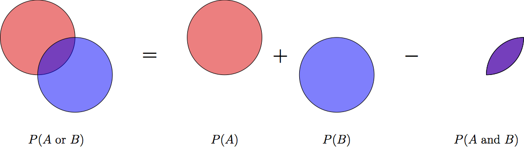
Figure 13.3: Graphical illustration of the general addition rule for probababilities.
13.7 Conditional probability
Conditional probability – is the probability that an event occurs given that a condition is met.
- Denoted: \(P(A|B)\). Read this as “the probability of A given B”or “the probability of A conditioned on B”.
13.7.1 Example: Conditional probability
Consider our urns and balls example, in which we make three draws (without replacement) from an urn filled with three white balls and two black balls.
The initial probability of drawing a black ball, P(B) = 2/5 = 0.4
If the first draw was a white ball, the probability of drawing a black ball is now, P(B|1st ball was white) = 2/4 = 0.5
13.8 General multiplication rule
The general form of the multiplication rule is: \[ P(A\ \text{and}\ B) = P(A)P(B|A) \]
13.8.1 Example: General multiplication rule
Consider our urns and balls example again. What is the probability that you draw, without replacement, three balls and they’re all white?
- The initial probability of drawing a white ball in the first draw is P(W) = 3/5
- The probability of drawing a white ball in the second draw, conditional on the first ball being white is P(W|1st White) = 1/2
- Therefore the P(1st White and 2nd White) = P(W)P(W|first White) = 3/10
- The probability of drawing a white ball in the third draw, conditional on the first two balls being white is P(W|1st White and 2nd White) = 1/3
- Therefore the P(1st White and 2nd White and 3rd White) = P(1st White and 2nd White)P(W|1st White and 2nd White) = (3/10)(1/3) = 1/10
13.9 Probability trees
Probability trees are diagrams that help calculate the probabilities of combinations of events across multiple random trials. A probability tree for the urns and balls example follows below.

Figure 13.4: Probability tree for the urns and balls example
The nodes in a probability tree represent the possible outcomes of each random trial. A path from the root node to one of the tips of the probability tree represents a sequence of outcomes resulting from the successive random trials. Along the edges of the probability tree we write the probability of each outcome for each trial. The probability of a specific sequence of outcomes is calculated by multiplying the probabilities along the path that represents that sequence.
To solve the problem we looked at previously – the probability of getting all white balls in three draws from the urn without replacement – we find all the sequences that yield this outcome. In this case there is only one sequence that results in three white balls. The product of the probabilities along the path representing this sequence is \(3/5 \times 2/4 \times 1/3 = 1/10\).
Another way to think about a probability tree is that values along the branches at a given point in the tree represent the conditional probabilities of the next possible outcomes, given all the previous outcomes.